A sample project: Zipf’s law¶

Let’s look at how we can use the suggested organization in a real project. We use the example of calculating Zipf’s law for a series of English texts, which was suggested in the book Research Software Engineering in Python, and was released under a CC-BY license. You can see the completed project on Github at github.com/patrickmineault/zipf.

What is Zipf’s law, anyway?¶

Zipf’s law comes from quantitative linguistics. It states the most used word in a language is used twice as much as the second most used word, three times as much of the third, etc. It’s an empirical law that holds in different languages and texts. There’s a lot of interesting theories about why it should hold - have a look at the Wikipedia article if you’re curious. A generalized form of Zipf’s law states that:

\[p(r) = \frac{1}{Cr^\alpha}\]

That is, the frequency of \(r^{th}\) most frequent word in a language is a power law with exponent \(\alpha\); the canonical Zipf’s law is obtained when \(\alpha=1\). \(C\) is a constant that makes the distribution add up to 1.

Our project¶

The goal of the project is to measure that Zipf’s law holds in three freely available texts. We’ll proceed as follows:

download some texts from project Gutenberg
compute the distribution of words
fit Zipf’s law to each of them
output metrics
plot some diagnostics

Let’s consider different ways to organize the different subcomponents and define how they should interact with each other. It’s clear that the processing has the nice structure of a (linear) directed acyclic graph (DAG).

Fig. 13 The Zipf project can be described as a linear directed acyclic graph (DAG)¶

Approach 1. We could make each box a separate script with command line arguments. Each script would be backed with module code that would help in a common library. Then, we would glue these scripts together with a bash file, or perhaps with make. This approach has a lot of merit, and in fact was the one that was originally suggested by the book: it’s clean and it’s standardized. One inconvenience is that it involves writing a lot of repetitive code in order to define command line interfaces. There’s also a bit of overhead in writing both a script and module code for each subcomponent.

Approach 2. We could make each box a separate function, held in a module. Then, we would glue these functions together with a Python script. This Python script would have its own command line arguments, which we could set in a bash script. One merit of the approach is that it has less overhead - fewer files and cruft - than the first approach.

The tradeoff between these two approaches lies in the balance between generality and complexity. The first is a bit more flexible than the second. We can’t run a single component of our analysis separately from the command line - we’ll need to implement tests instead, which feel a little less intuitive. If we wanted to run an analysis of tens of thousands of books, parallelizing would also be easier with the first approach (e.g. with make).

For this example, however, I have a slight preference for the second approach, so that’s the one we will implement. Keeping the number of command line tools to create to one means we’ll worry less about cruft and more about the computations. Let’s take a look at the DAG again to see how we’ll split the job:

Fig. 14 The Zipf project split into different sub-components.¶

We’ll create one module to compute the distribution of words, and another to fit Zipf’s law. We will create tests for each of those two modules. We’ll wrap the two modules as well as glue code inside a command line tool. Plotting will take place in jupyter notebook, which makes it easy to change plots interactively.

I encourage you to also have a look at the Python RSE github repo for an alternative implementation to examine the tradeoffs in different implementations.

Note

Most of the code is taken verbatim from the Py-RSE repo. Our emphasis here is on organizing project files.

Setup¶

Let’s proceed with setting up the project. zipf is a reasonable project name, so let’s go ahead and create a new project with that name:

(base) ~/Documents $ cookiecutter gh:patrickmineault/true-neutral-cookiecutter

Use zipf, zipf, and zipf as the answers to the first 3 questions, and “Zipf’s law project” as the description. Then proceed to create an environment and save it:

cd zipf
conda create --name zipf python=3.8
conda activate zipf
conda env export > environment.yml

Then we can sync to a Github remote. My favorite way of doing this is to use the GUI in vscode, which saves me from going to Github to create the remote and then type on the command line to sync locally. We can fire up vscode using:

code .

Then, in the git panel, we hit “Publish to Github” to locally set up git and create the Github remote in one shot.

Now we have a good looking project skeleton! We can set up black in vscode so that whenever a file is saved, it is formatted in a standard way. Time to add some code to it.

Note

If you prefer, you can instead go through github.com to create a new repo and follow the command line instructions there.

Download the texts¶

We want to download three texts and put them in the data folder. Ideally, we’d do this automatically, for example with a bash file with calls to wget. However, the terms and conditions from Project Gutenberg state:

The website is intended for human users only. Any perceived use of automated tools to access the Project Gutenberg website will result in a temporary or permanent block of your IP address. – Project Gutenberg

Caution

Document manual steps in README.md!

Not a big deal! We can download the files manually and document the source in the README.md file. Let’s download the following files manually and put them in the data folder:

Dracula \(\rightarrow\) data/dracula.txt
Frankenstein \(\rightarrow\) data/frankenstein.txt
Jane Eyre \(\rightarrow\) data/jane_eyre.txt

Count the words¶

The next step is to calculate word counts for each text. We will create a module called parse_text in the zipf folder. It will contain a function count_words that takes in a text string and outputs a set of counts. This function will itself call a helper function _clean_gutenberg_text. Note that the function starts with an underscore to indicate that it is meant to be a private function used internally by the module.

_clean_gutenberg_text will explicitly filter out boilerplate from project Gutenberg texts. There’s a significant amount of boilerplate at the start of e-books and license information at the end, which might skew the word count distribution. Thankfully, there are phrases in the e-books which delimit the main text, which we can detect:

START OF THE PROJECT GUTENBERG EBOOK
END OF THE PROJECT GUTENBERG EBOOK

Because we only have three books in our collection, we can manually test that each book is processed correctly. However, if we ever process a fourth, unusually formatted text, and our detection didn’t work, we want our pipeline to fail in a graceful way. Thus, we add in-line assert statements to make sure our filter finds the two delimiters in reasonable locations in the text.

def _clean_gutenberg_text(text):
    """
    Find fences in a Gutenberg text and select the text between them.
    """
    start_fence = "start of the project gutenberg ebook"
    end_fence = "end of the project gutenberg ebook"
    text = text.lower()
    start_pos = text.find(start_fence) + len(start_fence) + 1
    end_pos = text.find(end_fence)

    # Check that the fences are at reasonable positions within the text.
    assert 0.000001 < start_pos / len(text) <= 0.1
    assert 0.9 < end_pos / len(text) <= 1.0

    return text[start_pos:end_pos]

Now we can use call this function in another wrapper function that counts words ike so:

import string
import collections


def count_words(f, clean_text=False):
    """
    Count words in a file.

    Arguments:
        f: an open file handle
        clean_text (optional): a Boolean, if true, filters out boilerplate
            typical of a Gutenberg book.

    Returns:
        A dict keyed by word, with word counts
    """
    text = f.read()
    if clean_text:
        text = _clean_gutenberg_text(text)

    chunks = text.split()
    npunc = [word.strip(string.punctuation) for word in chunks]
    word_list = [word.lower() for word in npunc if word]
    word_counts = collections.Counter(word_list)
    return dict(word_counts)

To test that the count_words function works as intended, we make a sample txt file in the tests folder which contains dummy data:

The

*** START OF THE PROJECT GUTENBERG EBOOK ***
OF
TO to
I i i
and and and and
THE The     THE the thE
[...]
*** END OF THE PROJECT GUTENBERG EBOOK ***


OF

If our function works correctly, it should ignore all the text outside of the start and end fences. It should return:

{'the': 5, 'and': 4, 'i': 3, 'to': 2, 'of': 1}

We set up a test function in test_parse_text.py that loads this test text and verifies that the word counts are correctly measured. The test can be run with:

$ pytest tests/test_parse_text.py

The resulting module and test can be viewed on Github.

Calculate Zipf’s law¶

Once we have word counts, we can calculate Zipf’s law based on word counts. We use the method proposed in Moreno-Sanchez et al. (2016), which is implemented in the book Research Software Engineering with Python. The method calculates the maximum likelihood \(\alpha\) parameter for the empirical distribution of ranks. It starts with \(\alpha = 1\) and refines the estimate through gradient descent. We implement this method in fit_distribution.py.

It’s quite easy to make a mistake in calculating the exponent by incorrectly implementing the error function. To protect ourselves against this, in our test suite, we generate data from a known distribution with \(\alpha = 1\) and verify that the correct exponent is estimated. We put this test, test_fit_distribution.py under the tests folder.

Write the command line interface¶

We are now ready to write glue code to run our pipeline from the command line. We create a script, run_analysis.py, under the scripts folder. Our script takes in two different command line arguments, or flags:

in_folder: the input folder containing txt files.
out_folder: where we will output the results

We create this command line interface using argparse. This looks like this:

if __name__ == "__main__":
    parser = argparse.ArgumentParser(description="Compute zipf distribution")
    parser.add_argument("--in_folder", help="the input folder")
    parser.add_argument("--out_folder", help="the output folder")
    args = parser.parse_args()

    main(args)

The main function first verifies that there are files to be processed and creates the output folder if necessary. To manipulate paths, it uses the pathlib module. The function then runs each of the stages of the pipeline in turn until completion. We don’t write tests this part of the code, as we’ve lifted the error-prone aspects of the code elsewhere. Again, the goal is rarely to get 100% coverage, but rather to have good coverage where it counts.

The code uses a for loop to construct a table of results, which is then loaded into pandas, and then dumped to disk as csv. Pandas is not strictly necessary to write a csv file, but it’s the default choice to work with tabular data in Python, so it is used here. Have a look at the script here.

Make summary figures¶

Finally, to generate figures, we prefer the jupyter notebook environment. Polishing figures takes some trial and error, and the jupyter notebook environment makes it easy to iterate on figures. The notebook, in scripts/visualize_results.ipynb, takes in results files as csvs, and generates figures and summary tables from them.

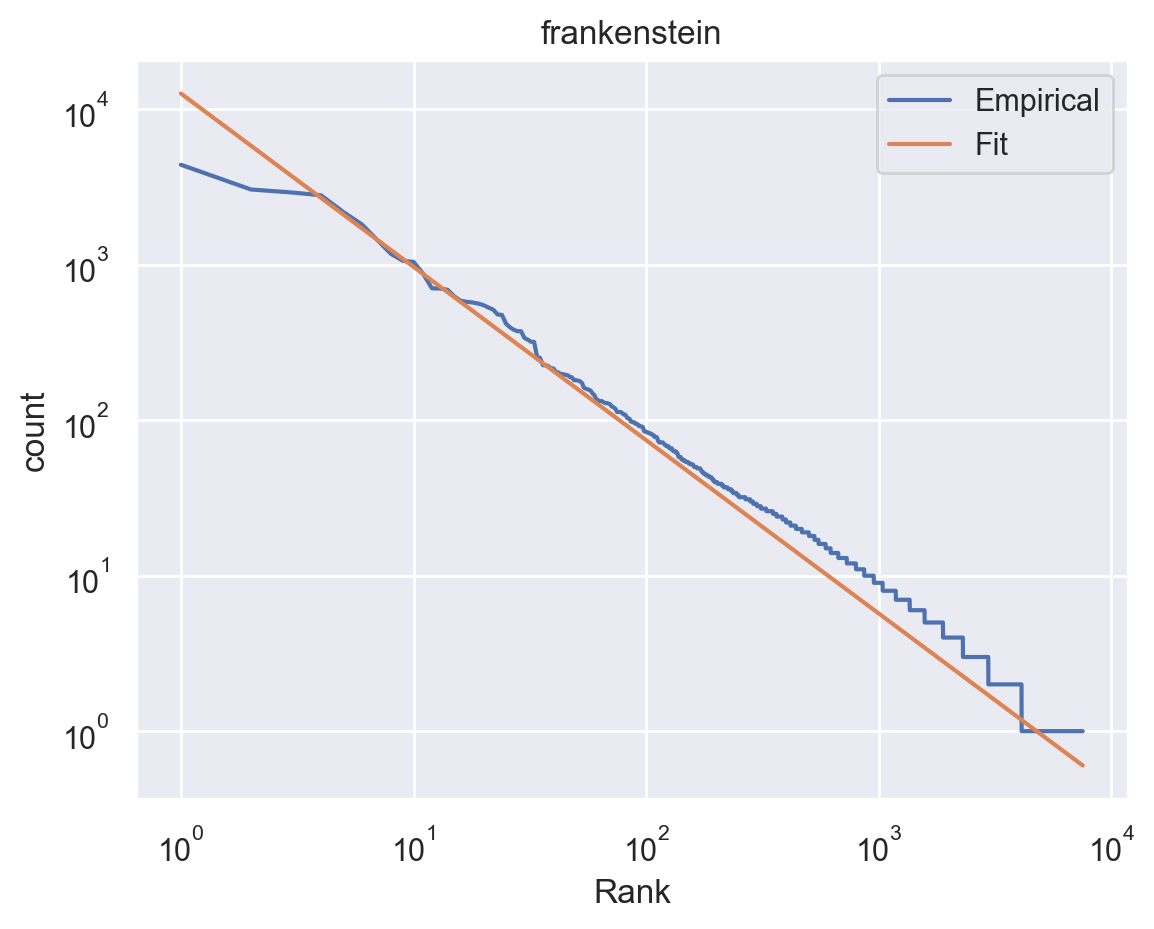
Fig. 15 A plot generated by our pipeline. Zipf distribution estimated on the novel Frankenstein by Mary Shelley.¶

We used the standard choice of matplotlib for the figures, although with the stylesheet from seaborn, which is more aesthetically pleasing. Note, however, that there are a number of excellent libraries for interactive graphics, so if this was critical, we could certainly apply this here. There is no computation in the notebook, only figure and summary table generation, which keeps the code in the notebook to a minimum.

What did we learn?¶

We saw how to organize an analysis according to the organization proposed in this handbook. We created a new project folder and module with the true neutral cookiecutter. If this analysis were part of a larger project - a paper or book chapter - we would re-use the same project folder, and add new pipelines and analyses to the project.

When I started this project, I was surprised by how many macro- and micro-decisions were needed to be made about how a pipeline works and how it’s organized. A little bit of thinking ahead can avoid days of headaches later on. In this case, we chose a lightweight structure with one entry script calling module functions. These module functions are short and most of them are pure functions. Pure functions are easier to test. Indeed, we wrote unit tests to check that these functions worked as intended. That way, once the code was written and tests passed, it was crystal clear that the code worked as intended. We separated module code from glue code and plotting code. The resulting code is decoupled and easily maintainable.

Writing code in this organized way is effortful. Over the long term, this methodical approach is more efficient, and more importantly, it’s less stressful.

5-minute exercise

How would you change this pipeline so that it computes error bars for the parameters of the Zipf distribution through bootstrapping? Would you need to change existing functions? What function would you need to add? If you’re feeling adventurous, go ahead and implement it! It’s definitely more than a 5-minute project!

Good research code