
Document your project
Research code is written in spurts and fits. You will often put code aside for several months and focus your energy on experiments, passing qualifying exams or working on another project. When you come back to your original project, you will be lost. A little prep work by writing docs will help you preserve your knowledge over the long run. In the previous chapter, I showed how to document small units of your code. In this section, I talk about how to document entire projects.
Document pipelines
It’s a common practice to use graphical tools (GUIs) to perform analyses. It also happens more often than most people are willing to admit that different variants of a pipeline are run by commenting and un-commenting code. Both of these practices make it hard to reproduce a result 6 months down the line. What was run, and when?
One approach is to textually document in detail what piece of code was run to obtain results. This method can be tedious and error-prone. It’s usually worth it to push as much computation as possible into reproducible pipelines which are self-documenting. That way, there’s no ambiguity about how results were produced.
Manual steps involving GUI tools should produce results which can be ingested by text-based pipelines. For instance, a interactive GUI to define regions-of-interest (ROI) should export the ROI coordinates in a way that the pipeline can ingest it.
Write console programs
Instead of commenting and un-commenting code, we can have different code paths execute depending on flags passed as command line arguments. Console programs can be written through the argparse library, which is part of the Python standard library, or through external libraries like click. As a side benefit, these libraries document the intent of the flags and generate help for them.
Let’s say you create a command line program train_net.py that trains a neural net. This training script has four parameters you could change: model type, number of iterations, input directory, output directory. Rather than changing these variables in the source code, you can pass them as command line arguments. Here’s how you can write that:
import argparse

def main(args):
    # TODO(pmin): Implement a neural net here.
    print(args.model)  # Prints the model type.

if __name__ == '__main__':
    parser = argparse.ArgumentParser(description="Train a neural net")

    parser.add_argument("--model", required=True,
      help="Model type (resnet or alexnet)")
    parser.add_argument("--niter", type=int, default=1000,
      help="Number of iterations")
    parser.add_argument("--in_dir", required=True,
      help="Input directory with images")
    parser.add_argument("--out_dir", required=True,
      help="Output directory with trained model")

    args = parser.parse_args()
    main(args)
A nice side benefit of using argparse is that it automatically generates help at the command line.
$ python train_net.py -h
usage: train_net.py [-h] --model MODEL [--niter NITER] --in_dir IN_DIR --out_dir OUT_DIR

Train a neural net

optional arguments:
  -h, --help         show this help message and exit
  --model MODEL      Model type (resnet or alexnet)
  --niter NITER      Number of iterations
  --in_dir IN_DIR    Input directory with images
  --out_dir OUT_DIR  Output directory with trained model
External flags thus allow you to run different versions of the same script in a standardized way.
Commit shell files
Once you’ve refactored your code to take configuration as command line flags, you should record the flags that you used when you invoke your code. You can do this using a shell file. A shell file contains multiple shell commands that are run one after the other.
Consider a long-running pipeline involving train_net.py. This pipeline starts with downloading images from the internet stored in an AWS S3 bucket; trains a neural net; then generates plots. We can document this pipeline with a shell file. In pipeline.sh, we have:
#!/bin/bash

# This will cause bash to stop executing the script if there's an error
set -e

# Download files
aws s3 cp s3://codebook-testbucket/images/ data/images --recursive

# Train network
python scripts/train_net.py --model resnet --niter 100000 --in_dir data/images \
  --out_dir results/trained_model

# Create output directory
mkdir results/figures/

# Generate plots
python scripts/generate_plots.py --in_dir data/images \
  --out_dir results/figures/ --ckpt results/trained_model/model.ckpt
This shell file serves both as runnable code and as documentation for the pipeline. Now we know how our figure was generated! Don’t forget to check in this shell file to git to have a record of this file.
Danger
Bash is quirky - the syntax is awkward and it’s pretty easy to shoot yourself in the foot. If you’re going to write elaborate shell scripts, use shellcheck, which will point out common mistakes in your code. Your favorite editor probably has a plugin for shellcheck.
Also, check out Julia Evans’ zine on bash - it’s a life saver.
Document pipelines with make
Scientific pipelines often take the shape of DAGs - directed acyclic graphs. This means, essentially, that programs flow from inputs to output in a directed fashion. The train_net pipeline above is a DAG with 4 steps. Other DAGs can be more elaborate, for example the 12-step DAG which generates figures shown in Van Vliet (2020) 1:
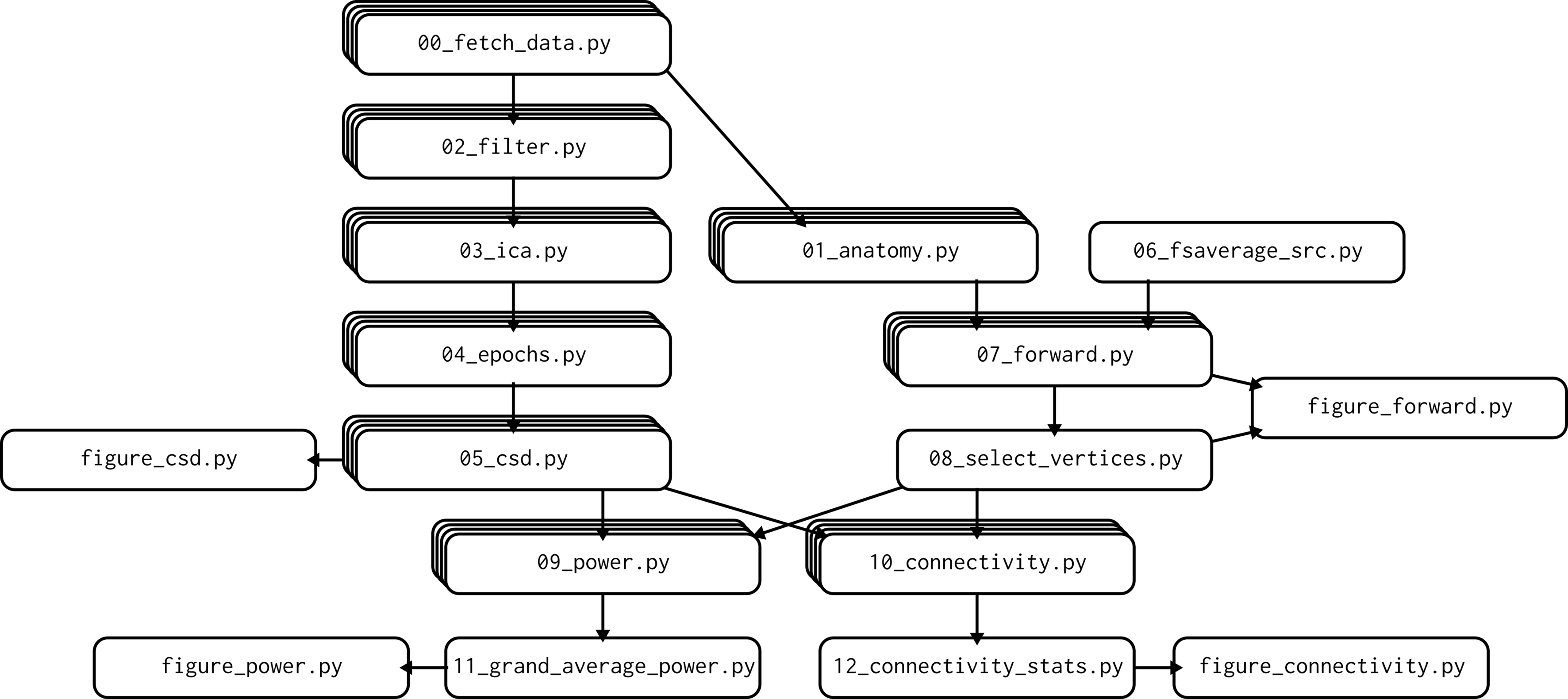
Fig. 11 DAG from Van Vliet (2020). CC-BY 4.0
You can document how all the steps of the DAG fit together with a bash file. As your pipelines grow, it can be painful to restart a pipeline that fails in the middle. This could lead to a proliferation of bash files corresponding to different subparts of your pipeline, and pretty soon you’ll have a mess of shell scripts on your hands - basically recreating the commenting/uncommenting workflow we had in Python, this time in bash!
You can use a more specialized build tool to build and document a pipeline. GNU make has been a standard tool for compiling code for several decades, and is becoming more adopted by the data science and research communities. A Makefile specifies both the inputs to each pipeline step and its outputs. To give you a flavor of what a Makefile looks like, this file implements the DAG to train a neural net and plot diagnostic plots:
.PHONY: plot
plot: results/trained_model/model.ckpt results/figures
  python scripts/generate_plots.py --in_dir data/images --out_dir \
    results/figures/ --ckpt results/trained_model/model.ckpt

results/trained_model/model.ckpt: data/images
  python scripts/train_net.py --model resnet --niter 100000 \
    --in_dir data/images --out_dir results/trained_model

data/images:
  aws s3 cp s3://codebook-testbucket/images/ data/images --recursive

results/figures:
  mkdir results/figures/
The plot can be created with make plot. The Makefile contains a complete description of the inputs and outputs to different scripts, and thus serves as a self-documenting artifact. Software carpentry has an excellent tutorial on make. What’s more, make only rebuilds what needs to be rebuilt. In particular, if the network is already trained, make will detect it and won’t retrain the network again, skipping ahead to the plotting task.
make uses a domain-specific language (DSL) to define a DAG. It might feel daunting to learn yet another language to document a pipeline. There are numerous alternatives to make that define DAGs in pure Python, including doit. There are also more complex tools that can implement Python DAGs and run them in the cloud, including luigi, airflow, and dask.
Record the provenance of each figure and table
Before you submit a manuscript, you should create a canonical version of the pipeline used to generate the figures and tables in the paper, and re-run the pipeline from scratch. That way, there will be no ambiguity as to the provenance of a figure in the final paper - it was generated by the canonical version of the pipeline.
However, before you get to this final state, it’s all too easy to lose track of which result was generated by which version of the pipeline. It is extremely frustrating when your results change and you can’t figure out why. If you check in figures and results to source control as you generate them, in theory you have access to a time machine. However, there’s information embedded in figures and tables about the state of the code when the figures were generated, only about the state of the code when the figures were committed, and there can be a significant lag between the two.
A lightweight workaround is to record the git hash with each result. The git hash is a long string of random digits corresponding to a git commit. You can see these hashes using git log:
$ git log
commit 3b0c0665465a8ea4cd862058e107b76041acae0f (HEAD -> main, origin/main)
Author: Patrick Mineault <patrick.mineault@gmail.com>
Date:   Wed Sep 8 13:34:31 2021 -0400

    Clean up setup instructions

commit 70deb0e7c9bffe4cdc73d813df8115d99606601c
Author: Patrick Mineault <patrick.mineault@gmail.com>
Date:   Wed Sep 8 00:41:10 2021 -0400
Here, 3b0c06... is the git hash of my latest commit. You can read the current git hash using the gitpython library and append it to the name of file. For example, instead of recording figure.png, I can record figure.3b0c066546.png using:
import git
import matplotlib.pyplot as plt

repo = git.Repo(search_parent_directories=True)
short_hash = repo.head.object.hexsha[:10]

# Plotting code goes here...
plt.savefig(f'figure.{short_hash}.png')
Now there’s no ambiguity about how that figure was generated. You can repeat the same process with csv files and other results.
A more full-featured way of doing this is to use a specialized tool to post results to a centralized database. Most of the offerings in this space are cloud-based commercial services. You post your results - whether scalars, whole tables, figures, etc. - to a centralized server through a bit of python code, and it takes care of versioning. In the screenshot below, I used wandb.ai to record the outcome of a machine learning pipeline. The record tells me what command that was run, the git hash, meta-information about which computer was used to run the pipeline, as well as the outcome. There is no ambiguity about provenance.
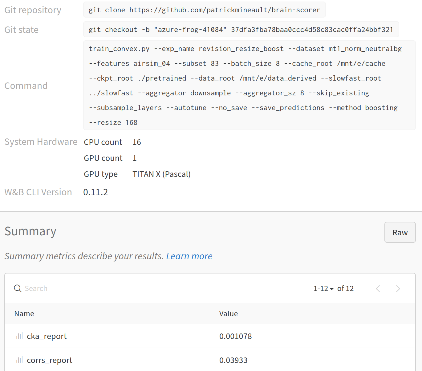
Fig. 12 Record of one deep-learning run in wandb.ai
Document projects
In addition to documenting pipelines, it’s important to write proper textual documentation for your project. The secret is that once you’ve written good unit tests and have documented your pipelines, you won’t have a lot of text docs to write.
Write a README.md file
README.md is the often first entry point to your code that you and others will see. This is the file that’s rendered when you navigate to your git repository. What are some of the elements in a good README?
A one-sentence description of your project
A longer description of your project
Installation instructions
General orientation to the codebase and usage instructions
Links to papers
Links to extended docs
License
Importantly, keep your README.md up-to-date. A good README.md file helps strangers understand the value of your code: it’s as important as a paper’s abstract.
Write Markdown docs
Markdown has taken over the world of technical writing. Using the same format everywhere creates tremendous opportunities, so I highly recommend that you write your documentation in Markdown. With the same text, you can generate:
Wikis. GitHub.
Executable books. jupyterbook generates this book.
Papers. CurveNote uses MyST Markdown under the hood.
Slide decks. Pandoc via conversion to LaTeX/Beamer.
readthedocs-style documentation. Sphinx using MyST.
The same Markdown can be deployed in different environments depending on what exactly you want to accomplish. For some projects, the README.md file will be all that is needed. Others will want a static site that shows highlights of the paper. Yet other projects will be well-served by blog posts which discuss in longer form the tradeoffs involved in the design decisions.
Creating your documentation in Markdown you make it really easy for you to eventually migrate to another format. I tend to use a combination of all these tools. For instance, I write notes on papers in Notion; I then export those notes to markdown as stubs for my Wordpress blog, for pandoc slides or for jupyterbook.
Discussion
Some things are in our control and others not. […] If [a thing] concerns anything not in your control, be prepared to say that it is nothing to you.
—Epictetus
Documentation contains the long-term memory of a project. When you’re writing documentation, you’re ensuring that your code will remain useful for a long time. Code should be self-documenting to a large degree, and you should put effort into automating most of the steps involved in generating figures and tables in your paper. However, you will still need to write some textual documentation.
You can take that occasion to reflect on your project. Sometimes, you’ll find that it’s more productive to rewrite bad code than to write complex explanations for it. At other times, especially at the very end of a project, refactoring will not be worth the effort, and you will have to let things go. As part of the documentation, you can write about how you could improve on your project. You can use a framing device device like three lessons I learned in this project. Learn from your mistakes and do better next time.
5-minute exercise
Add a README.md file to a project you’re working on right now
- 1
Van Vliet (2020). Seven quick tips for analysis scripts in neuroimaging. PLOS Computational Biology.